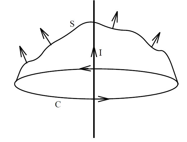
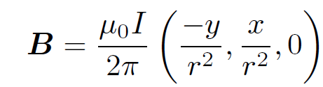
Consider, again, an infinite straight wire aligned along the z-axis and carrying a current I. The field generated by such a wire is written

 (1.1)

in cylindrical polar coordinates. Consider a circular loop C in the x-y plane which is centred on the wire. Suppose that the radius of this loop is r. Let us evaluate the line integral  B . dl. This integral is easy to perform because the magnetic field is always parallel to the line element. We have

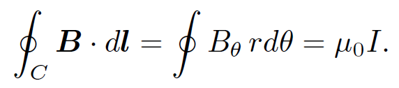 (1.2)

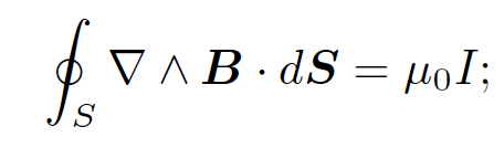
However, we know from Stokes' theorem that

 (1.3)

where S is any surface attached to the loop C. Let us evaluate ∇ ˄ B directly.

According to

:

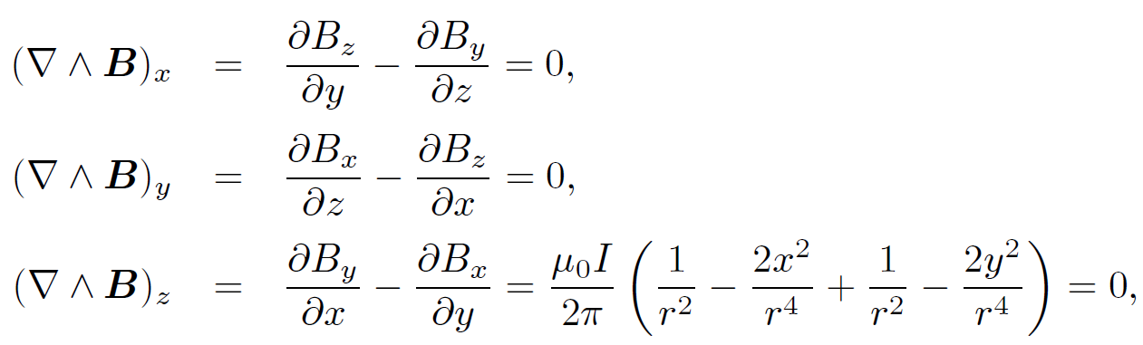 (1.4)

where use has been made of ∂r/∂x = x/r, etc. We now have a problem. Equations (1.2) and (1.3) imply that

 (1.5)

but we have just demonstrated that ∇ ˄ B = 0. This problem is very reminiscent of the difficulty we had earlier with ∇ ˄ E. Recall that ∫_V ∇ ˄ E dV = q/ for a volume V containing a discrete charge q, but that ∇ ˄ E = 0 at a general point. We got around this problem by saying that ∇ ˄ E is a three-dimensional delta function whose ''spike" is coincident with the location of the charge. Likewise, we can get around our present difficulty by saying that ∇ ˄ B is a two-dimensional delta function. A three-dimensional delta-function is a singular (but integrable) point in space, whereas a two-dimensional delta-function is a singular line in space. It is clear from an examination of Eqs. (1.4) that the only component of ∇ ˄ B which can be singular is the z-component, and that this can only be singular on the z-axis (i.e., r = 0). Thus, the singularity coincides with the location of the current, and we can write

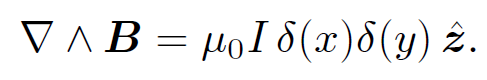 (1.6)

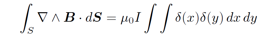
The above equation certainly gives (∇ ˄ B)_x = (∇ ˄ B)_y = 0, and (∇ ˄ B)_z = 0 everywhere apart from the z-axis, in accordance with Eqs. (1.4). Suppose that we integrate over a plane surface S connected to the loop C. The surface element is 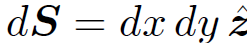, so

 (1.7)

where the integration is performed over the region . However, since the only part of S which actually contributes to the surface integral is the bit which lies infinitesimally close to the z-axis, we can integrate over all x and y without changing the result. Thus, we obtain

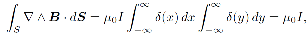 (1.8)

which is in agreement with Eq. (1.5). You might again be wondering why we have gone to so much trouble to prove something using vector field theory which can be demonstrated in one line via conventional analysis. The answer, of course, is that the vector field result is easily generalized whereas the conventional result is just a special case. For instance, suppose that we distort our simple circular loop C so that it is no longer circular or even lies in one plane. What now is the line integral of B around the loop? This is no longer a simple problem for conventional analysis, because the magnetic field is not parallel to the line element of the loop. However, according to Stokes' theorem

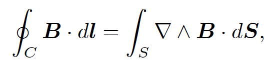 (1.9)

with ∇ ˄ B given by Eq. (1.6). Note that the only part of S which contributes to the surface integral is an infinitesimal region centered on the z-axis. So, as long as S actually intersects the z-axis it does not matter what shape the rest the surface is, we always get the same answer for the surface integral, namely

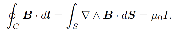 (1.10)

Thus, provided the curve C circulates the z-axis, and therefore any surface S attached to C intersects the z-axis, the line integral  B . dl is equal to μ₀I. Of course, if C does not circulate the z-axis then an attached surface S does not intersect the z-axis and  B . dl is zero. There is one more proviso. The line integral  B . dl is μ₀I for a loop which circulates the z-axis in a clockwise direction (looking up the z-axis). However, if the loop circulates in an anticlockwise direction then the integral is -μ₀I. This follows because in the latter case the z-component of the surface element dS is oppositely directed to the current flow at the point where the surface intersects the wire. Let us now consider N wires directed along the z-axis, with coordinates (x_i, y_i) in the x-y plane, each carrying a current Ii in the positive z-direction. It is fairly obvious that Eq. (1.6) generalizes to

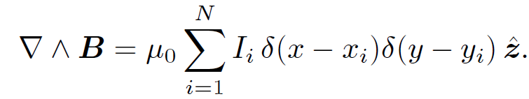 (1.11)

If we integrate the magnetic field around some closed curve C, which can have any shape and does not necessarily lie in one plane, then Stokes' theorem and the above equation imply that

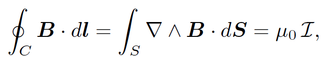 (1.12)

where  is the total current enclosed by the curve. Again, if the curve circulates the ith wire in a clockwise direction (looking down the direction of current flow) then the wire contributes I_i to the aggregate current . On the other hand, if the curve circulates in an anti-clockwise direction then the wire contributes -I_i. Finally, if the curve does not circulate the wire at all then the wire contributes nothing to . Equation (1.11) is a field equation describing how a set of z-directed current carrying wires generate a magnetic field. These wires have zero-thickness, which implies that we are trying to squeeze a finite amount of current into an infinitesimal region. This accounts for the delta-functions on the right-hand side of the equation. Likewise, we obtained delta-functions because we were dealing with point charges. Let us now generalize to the more realistic case of diffuse currents. Suppose that the z-current flowing through a small rectangle in the x-y plane, centred on coordinates (x, y) and of dimensions dx and dy, is j_z(x, y) dx dy. Here, j_z is termed the current density in the z-direction. Let us integrate (∇ ˄ B)_z over this rectangle. The rectangle is assumed to be sufficiently small that (∇ ˄ B)_z does not vary appreciably across it. According to Eq. (1.12) this integral is equal to μ₀ times the total z-current flowing through the rectangle. Thus,

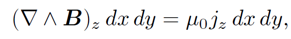 (1.13)

which implies that

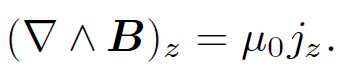 (1.14)

Of course, there is nothing special about the z-axis. Suppose we have a set of diffuse currents flowing in the x-direction. The current flowing through a small rectangle in the y-z plane, centred on coordinates (y, z) and of dimensions dy and dz, is given by j_x(y, z) dy dz, where j_x is the current density in the x-direction. It is fairly obvious that we can write

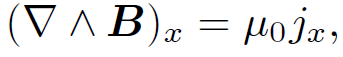 (1.15)

with a similar equation for diffuse currents flowing along the y-axis. We can combine these equations with Eq. (1.14) to form a single vector field equation which describes how electric currents generate magnetic fields:

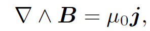 (1.16)

where j = (j_x, j_y, j_z) is the vector current density. This is the third Maxwell equation. The electric current °owing through a small area dS located at position r is j(r) . dS. Suppose that space is filled with particles of charge q, number density n(r), and velocity v(r). The charge density is given by ρ(r) = qn. The current density is given by j(r) = qn v and is obviously a proper vector field (velocities are proper vectors since they are ultimately derived from displacements). If we form the line integral of B around some general closed curve C, making use of Stokes' theorem and the field equation (1.16), then we obtain

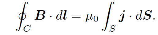 (1.17)

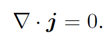
In other words, the line integral of the magnetic field around any closed loop C is equal to μ₀ times the flux of the current density through C. This result is called Ampere's (other) law. If the currents flow in zero-thickness wires then Ampere's law reduces to Eq. (1.12). The flux of the current density through C is evaluated by integrating j . dS over any surface S attached to C. Suppose that we take two different surfaces S₁ and S₂. It is clear that if Ampere's law is to make any sense then the surface integral ∫_S1 j . dS had better equal the integral ∫_S1 j . dS. That is, when we work out the flux of the current though C using two different attached surfaces then we had better get the same answer, otherwise Eq. (1.17) is wrong. We saw in

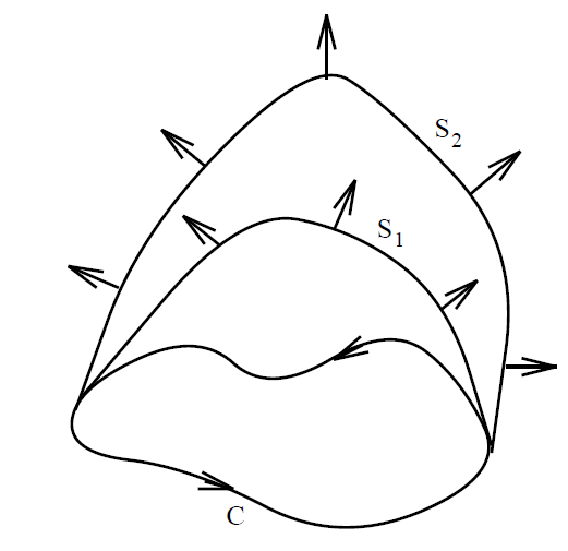
Section 2 that if the integral of a vector field A over some surface attached to a loop depends only on the loop, and is independent of the surface which spans it, then this implies that ∇ . A = 0. The flux of the current density through any loop C is calculated by evaluating the integral ∫_S j .dS for any surface S which spans the loop. According to Ampere's law, this integral depends only on C and is completely independent of S (i.e., it is equal to the line integral of B around C, which depends on C but not on S). This implies that ∇ . j = 0. In fact, we can obtain this relation directly from the field equation (1.16). We know that the divergence of a curl is automatically zero, so taking the divergence of Eq. (1.16) we obtain

 (1.18)

We have shown that if Ampere's law is to make any sense then we need ∇ . j = 0. Physically this implies that the net current flowing through any closed surface S is zero. Up to now we have only considered stationary charges and steady currents. It is clear that if all charges are stationary and all currents are steady then there can be no net current °owing through a closed surface S, since this would imply a build up of charge in the volume V enclosed by S. In other words, as long as we restrict our investigation to stationary charges and steady currents then we expect ∇ . j = 0, and Ampere's law makes sense. However, suppose that we now relax this restriction. Suppose that some of the charges in a volume V decide to move outside V . Clearly, there will be a non-zero net flux of electric current through the bounding surface S whilst this is happening. This implies from Gauss' theorem that ∇ . j ≠ 0. Under these circumstances Ampere's law collapses in a heap. We shall see later that we can rescue Ampere's law by adding an extra term involving a time derivative to the right-hand side of the field equation (1.16). For steady state situations (i.e., ∂/∂t = 0) this extra term can be neglected. Thus, the field equation ∇ ˄ B = μ₀ j is, in fact, only two-thirds of Maxwell's third equation; there is a term missing on the right-hand side. We have now derived two field equations involving magnetic fields (actually, we have only derived one and two-thirds):

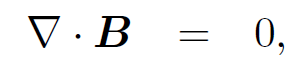 (1.19a)

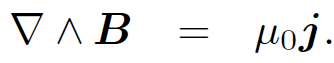 (1.19b)

We obtained these equations by looking at the fields generated by infinitely long, straight, steady currents. This, of course, is a rather special class of currents. We should now go back and repeat the process for general currents. In fact, if we did this we would find that the above field equations still hold (provided that the currents are steady). Unfortunately, this demonstration is rather messy and extremely tedious. There is a better approach. Let us assume that the above field equations are valid for any set of steady currents. We can then, with relatively little effort, use these equations to generate the correct formula for the magnetic field induced by a general set of steady currents, thus proving that our assumption is correct. More of this later.