آخر المواضيع المضافة

 تاريخ الرياضيات
الرياضيات في الحضارات المختلفة
الرياضيات المتقطعة
الجبر
الهندسة
المعادلات التفاضلية و التكاملية
التحليل
علماء الرياضيات
تاريخ الرياضيات
الرياضيات في الحضارات المختلفة
الرياضيات المتقطعة
الجبر
الهندسة
المعادلات التفاضلية و التكاملية
التحليل
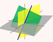
علماء الرياضيات | Bivariate Normal Distribution |


|
|
Read More
Date: 19-5-2019
Date: 22-6-2019
Date: 2-9-2019
|
The bivariate normal distribution is the statistical distribution with probability density function
 |
(1) |
where
 |
(2) |
and
 |
(3) |
is the correlation of  and
and  (Kenney and Keeping 1951, pp. 92 and 202-205; Whittaker and Robinson 1967, p. 329) and
  is the covariance.
The probability density function of the bivariate normal distribution is implemented as MultinormalDistribution[ mu1, mu2
 ,
, 
 sigma11, sigma12
 ,
,  sigma12, sigma22
 ] in the Wolfram Language package MultivariateStatistics` .
The marginal probabilities are then
 |
 |
 |
(4) |
 |
 |
 |
(5) |
and
 |
 |
 |
(6) |
 |
 |
 |
(7) |
(Kenney and Keeping 1951, p. 202).
Let  and
and  be two independent normal variates with means
  and
and  for
for  , 2. Then the variables
  and
and  defined below are normal bivariates with unit variance and correlation coefficient
  :
:
 |
 |
 |
(8) |
 |
 |
 |
(9) |
To derive the bivariate normal probability function, let  and
and  be normally and independently distributed variates with mean 0 and variance 1, then define
 |
 |
 |
(10) |
 |
 |
 |
(11) |
(Kenney and Keeping 1951, p. 92). The variates  and
and  are then themselves normally distributed with means
  and
and  , variances
 |
 |
 |
(12) |
 |
 |
 |
(13) |
and covariance
 |
(14) |
The covariance matrix is defined by
 |
(15) |
where
 |
(16) |
Now, the joint probability density function for  and
and  is
is
 |
(17) |
but from (◇) and (◇), we have
 |
(18) |
As long as
 |
(19) |
this can be inverted to give
![[x_1; x_2]](http://mathworld.wolfram.com/images/equations/BivariateNormalDistribution/Inline58.gif) |
 |
 |
(20) |
 |
 |
 |
(21) |
Therefore,
 |
(22) |
and expanding the numerator of (22) gives
 |
(23) |
so
 |
(24) |
Now, the denominator of (◇) is
 |
(25) |
so
 |
 |
 |
(26) |
 |
 |
 |
(27) |
 |
 |
 |
(28) |
can be written simply as
 |
(29) |
and
 |
(30) |
Solving for  and
and  and defining
 |
(31) |
gives
 |
 |
 |
(32) |
 |
 |
 |
(33) |
But the Jacobian is
 |
 |
 |
(34) |
 |
 |
 |
(35) |
 |
 |
 |
(36) |
so
 |
(37) |
and
 |
(38) |
where
 |
(39) |
Q.E.D.
The characteristic function of the bivariate normal distribution is given by
 |
 |
 |
(40) |
 |
 |
 |
(41) |
where
 |
(42) |
and
 |
(43) |
Now let
 |
 |
 |
(44) |
 |
 |
 |
(45) |
Then
 |
(46) |
where
 |
 |
![-1/(2(1-rho^2))1/(sigma_1^2)[u^2-(2rhosigma_1w)/(sigma_2)u]](http://mathworld.wolfram.com/images/equations/BivariateNormalDistribution/Inline104.gif) |
(47) |
 |
 |
 |
(48) |
Complete the square in the inner integral
 |
(49) |
Rearranging to bring the exponential depending on  outside the inner integral, letting
 |
(50) |
and writing
 |
(51) |
gives
 |
(52) |
Expanding the term in braces gives
 |
(53) |
But  is odd, so the integral over the sine term vanishes, and we are left with
 |
(54) |
Now evaluate the Gaussian integral
 |
 |
 |
(55) |
 |
 |
 |
(56) |
to obtain the explicit form of the characteristic function,
 |
(57) |
In the singular case that
 |
(58) |
(Kenney and Keeping 1951, p. 94), it follows that
 |
(59) |
 |
 |
 |
(60) |
 |
 |
 |
(61) |
 |
 |
 |
(62) |
 |
 |
 |
(63) |
so
 |
 |
 |
(64) |
 |
 |
 |
(65) |
where
 |
 |
 |
(66) |
 |
 |
 |
(67) |
The standardized bivariate normal distribution takes  and
and  . The quadrant probability in this special case is then given analytically by
 |
 |
 |
(68) |
 |
 |
 |
(69) |
 |
 |
 |
(70) |
(Rose and Smith 1996; Stuart and Ord 1998; Rose and Smith 2002, p. 231). Similarly,
 |
 |
 |
(71) |
 |
 |
 |
(72) |
 |
 |
 |
(73) |
REFERENCES:
Abramowitz, M. and Stegun, I. A. (Eds.). Handbook of Mathematical Functions with Formulas, Graphs, and Mathematical Tables, 9th printing. New York: Dover, pp. 936-937, 1972.
Holst, E. "The Bivariate Normal Distribution." http://www.ami.dk/research/bivariate/.
Kenney, J. F. and Keeping, E. S. Mathematics of Statistics, Pt. 2, 2nd ed. Princeton, NJ: Van Nostrand, 1951.
Kotz, S.; Balakrishnan, N.; and Johnson, N. L. "Bivariate and Trivariate Normal Distributions." Ch. 46 in Continuous Multivariate Distributions, Vol. 1: Models and Applications, 2nd ed. New York: Wiley, pp. 251-348, 2000.
Rose, C. and Smith, M. D. "The Multivariate Normal Distribution." Mathematica J. 6, 32-37, 1996.
Rose, C. and Smith, M. D. "The Bivariate Normal." §6.4 A in Mathematical Statistics with Mathematica. New York: Springer-Verlag, pp. 216-226, 2002.
Spiegel, M. R. Theory and Problems of Probability and Statistics. New York: McGraw-Hill, p. 118, 1992.
Stuart, A.; and Ord, J. K. Kendall's Advanced Theory of Statistics, Vol. 1: Distribution Theory, 6th ed. New York: Oxford University Press, 1998.
Whittaker, E. T. and Robinson, G. "Determination of the Constants in a Normal Frequency Distribution with Two Variables" and "The Frequencies of the Variables Taken Singly." §161-162 in The Calculus of Observations: A Treatise on Numerical Mathematics, 4th ed. New York: Dover, pp. 324-328, 1967.

|
|
|
|
15 نوعا من الأطعمة تساعدك على ترطيب جسمك خلال موجة الحر
|
|
|
|
|
|
|
"ناسا" تختار شركة "سبيس إكس" لـ"مهمة خاصة" في 2030
|
|
|
|
|
|
|
بالصور: بمناسبة عيد الغدير الاغر.. قراءة خطبة النبي الأكرم (ص وآله) بالمسلمين في يوم (غدير خم)
|
|
|