
آخر المواضيع المضافة

 الفيزياء الكلاسيكية
الكهربائية والمغناطيسية
علم البصريات
الفيزياء الحديثة
النظرية النسبية
الفيزياء النووية
فيزياء الحالة الصلبة
الليزر
علم الفلك
المجموعة الشمسية
الطاقة البديلة
الفيزياء والعلوم الأخرى
مواضيع عامة في الفيزياء
الفيزياء الكلاسيكية
الكهربائية والمغناطيسية
علم البصريات
الفيزياء الحديثة
النظرية النسبية
الفيزياء النووية
فيزياء الحالة الصلبة
الليزر
علم الفلك
المجموعة الشمسية
الطاقة البديلة
الفيزياء والعلوم الأخرى
مواضيع عامة في الفيزياء| Adding two waves |


|
|
أقرأ أيضاً
التاريخ: 2024-01-27
التاريخ: 2024-01-14
التاريخ: 17-5-2016
التاريخ: 17-5-2016
|
Suppose we have two equal oscillating sources of the same frequency whose phases are so adjusted, say, that the signals arrive in phase at some point P. At that point, if it is light, the light is very strong; if it is sound, it is very loud; or if it is electrons, many of them arrive. On the other hand, if the arriving signals were 180∘ out of phase, we would get no signal at P, because the net amplitude there is then a minimum. Now suppose that someone twists the “phase knob” of one of the sources and changes the phase at P back and forth, say, first making it 0∘ and then 180∘, and so on. Of course, we would then find variations in the net signal strength. Now we also see that if the phase of one source is slowly changing relative to that of the other in a gradual, uniform manner, starting at zero, going up to ten, twenty, thirty, forty degrees, and so on, then what we would measure at P would be a series of strong and weak “pulsations,” because when the phase shifts through 360∘ the amplitude returns to a maximum. Of course, to say that one source is shifting its phase relative to another at a uniform rate is the same as saying that the number of oscillations per second is slightly different for the two.
So we know the answer: if we have two sources at slightly different frequencies we should find, as a net result, an oscillation with a slowly pulsating intensity. That is all there really is to the subject!
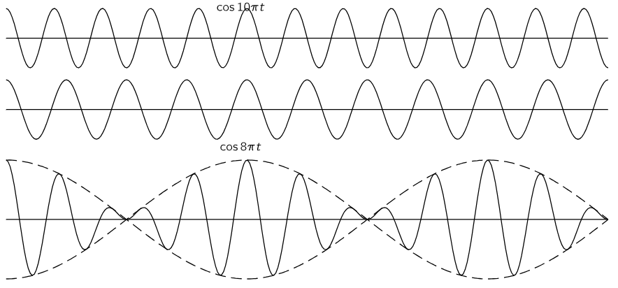
Fig. 48–1. The superposition of two cosine waves with frequencies in the ratio 8:10. The precise repetition of the pattern within each “beat” is not typical of the general case.
It is very easy to formulate this result mathematically also. Suppose, for example, that we have two waves, and that we do not worry for the moment about all the spatial relations, but simply analyze what arrives at P. From one source, let us say, we would have cosω1t, and from the other source, cosω2t, where the two ω’s are not exactly the same. Of course, the amplitudes may not be the same, either, but we can solve the general problem later; let us first take the case where the amplitudes are equal. Then the total amplitude at P is the sum of these two cosines. If we plot the amplitudes of the waves against the time, as in Fig. 48–1, we see that where the crests coincide, we get a strong wave, and where a trough and crest coincide, we get practically zero, and then when the crests coincide again, we get a strong wave again.
Mathematically, we need only to add two cosines and rearrange the result somehow. There exist a number of useful relations among cosines which are not difficult to derive. Of course, we know that
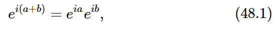
and that eia has a real part, cos a, and an imaginary part, sin a. If we take the real part of ei(a+b), we get cos (a+b). If we multiply out:

we get cos a cos b – sin a sin b, plus some imaginary parts. But we now need only the real part, so we have

Now if we change the sign of b, since the cosine does not change sign while the sine does, the same equation, for negative b, is

If we add these two equations together, we lose the sines and we learn that the product of two cosines is half the cosine of the sum, plus half the cosine of the difference:

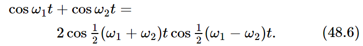
Now we can also reverse the formula and find a formula for cos α+cos β if we simply let α=a+b and β=a−b. That is, a=1/2(α+β) and b=1/2(α−β), so that

Now we can analyze our problem. The sum of cosω1t and cosω2t is
Now let us suppose that the two frequencies are nearly the same, so that 1/2(ω1+ω2) is the average frequency, and is more or less the same as either. But ω1−ω2 is much smaller than ω1 or ω2 because, as we suppose, ω1 and ω2 are nearly equal. That means that we can represent the solution by saying that there is a high-frequency cosine wave more or less like the ones we started with, but that its “size” is slowly changing—its “size” is pulsating with a frequency which appears to be 1/2 (ω1−ω2). But is this the frequency at which the beats are heard? Although (48.6) says that the amplitude goes as cos1/2(ω1−ω2)t, what it is really telling us is that the high-frequency oscillations are contained between two opposed cosine curves (shown dotted in Fig. 48–1). On this basis one could say that the amplitude varies at the frequency 1/2(ω1−ω2), but if we are talking about the intensity of the wave we must think of it as having twice this frequency. That is, the modulation of the amplitude, in the sense of the strength of its intensity, is at frequency ω1−ω2, although the formula tells us that we multiply by a cosine wave at half that frequency. The technical basis for the difference is that the high frequency-wave has a little different phase relationship in the second half-cycle.
Ignoring this small complication, we may conclude that if we add two waves of frequency ω1 and ω2, we will get a net resulting wave of average frequency 1/2(ω1+ω2) which oscillates in strength with a frequency ω1−ω2.
If the two amplitudes are different, we can do it all over again by multiplying the cosines by different amplitudes A1 and A2, and do a lot of mathematics, rearranging, and so on, using equations like (48.2)–(48.5). However, there are other, easier ways of doing the same analysis. For example, we know that it is much easier to work with exponentials than with sines and cosines and that we can represent A1cosω1t as the real part of A1eiω1t. The other wave would similarly be the real part of A2eiω2t. If we add the two, we get A1eiω1t+A2eiω2t. If we then factor out the average frequency, we have
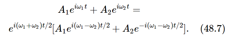
Again we have the high-frequency wave with a modulation at the lower frequency.


|
|
|
|
4 أسباب تجعلك تضيف الزنجبيل إلى طعامك.. تعرف عليها
|
|
|
|
|
|
|
أكبر محطة للطاقة الكهرومائية في بريطانيا تستعد للانطلاق
|
|
|
|
|
|
|
العتبة العباسية المقدسة تبحث مع العتبة الحسينية المقدسة التنسيق المشترك لإقامة حفل تخرج طلبة الجامعات
|
|
|