آخر المواضيع المضافة

 الفيزياء الكلاسيكية
الكهربائية والمغناطيسية
علم البصريات
الفيزياء الحديثة
النظرية النسبية
الفيزياء النووية
فيزياء الحالة الصلبة
الليزر
علم الفلك
المجموعة الشمسية
الطاقة البديلة
الفيزياء والعلوم الأخرى
مواضيع عامة في الفيزياء
الفيزياء الكلاسيكية
الكهربائية والمغناطيسية
علم البصريات
الفيزياء الحديثة
النظرية النسبية
الفيزياء النووية
فيزياء الحالة الصلبة
الليزر
علم الفلك
المجموعة الشمسية
الطاقة البديلة
الفيزياء والعلوم الأخرى
مواضيع عامة في الفيزياء| The field of a plane of oscillating charges |


|
|
أقرأ أيضاً
التاريخ: 2024-03-20
التاريخ: 28-11-2019
التاريخ: 2024-01-10
التاريخ: 2024-03-17
|
Suppose that we have a plane full of sources, all oscillating together, with their motion in the plane and all having the same amplitude and phase. What is the field at a finite, but very large, distance away from the plane? (We cannot get very close, of course, because we do not have the right formulas for the field close to the sources.) If we let the plane of the charges be the xy-plane, then we want to find the field at the point P far out on the z-axis (Fig. 30–10). We suppose that there are η charges per unit area of the plane, and that each one of them has a charge q. All of the charges move with simple harmonic motion, with the same direction, amplitude, and phase. We let the motion of each charge, with respect to its own average position, be x0 cos ωt. Or, using the complex notation and remembering that the real part represents the actual motion, the motion can be described by x0eiωt.
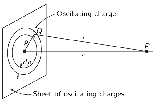
Fig. 30–10. Radiation field of a sheet of oscillating charges.
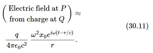
Now we find the field at the point P from all of the charges by finding the field there from each charge q, and then adding the contributions from all the charges. We know that the radiation field is proportional to the acceleration of the charge, which is −ω2x0eiωt (and is the same for every charge). The electric field that we want at the point P due to a charge at the point Q is proportional to the acceleration of the charge q, but we have to remember that the field at the point P at the instant t is given by the acceleration of the charge at the earlier time t′=t−r/c, where r/c is the time, it takes the waves to travel the distance r from Q to P. Therefore, the field at P is proportional to

Using this value for the acceleration as seen from P in our formula for the electric field at large distances from a radiating charge, we get
Now this formula is not quite right, because we should have used not the acceleration of the charge but its component perpendicular to the line QP. We shall suppose, however, that the point P is so far away, compared with the distance of the point Q from the axis (the distance ρ in Fig. 30–10), for those charges that we need to take into account, that we can leave out the cosine factor (which would be nearly equal to 1 anyway).
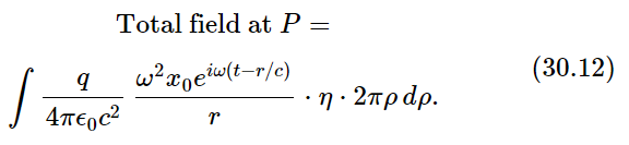
To get the total field at P, we now add the effects of all the charges in the plane. We should, of course, make a vector sum. But since the direction of the electric field is nearly the same for all the charges, we may, in keeping with the approximation we have already made, just add the magnitudes of the fields. To our approximation the field at P depends only on the distance r, so all charges at the same r produce equal fields. So, we add, first, the fields of those charges in a ring of width dρ and radius ρ. Then, by taking the integral over all ρ, we will obtain the total field.
The number of charges in the ring is the product of the surface area of the ring, 2π ρ dρ, and η, the number of charges per unit area. We have, then,
We wish to evaluate this integral from ρ=0 to ρ=∞. The variable t, of course, is to be held fixed while we do the integral, so the only varying quantities are ρ and r. Leaving out all the constant factors, including the factor eiωt, for the moment, the integral we wish is
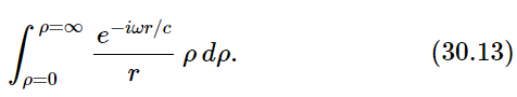
To do this integral we need to use the relation between r and ρ:
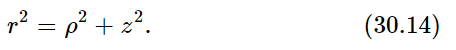
Since z is independent of ρ, when we take the differential of this equation, we get
2r dr = 2ρ dρ,
which is lucky, since in our integral we can replace ρ dρ by r dr and the r will cancel the one in the denominator. The integral we want is then the simpler one
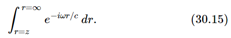
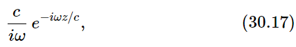
To integrate an exponential is very easy. We divide by the coefficient of r in the exponent and evaluate the exponential at the limits. But the limits of r are not the same as the limits of ρ. When ρ=0, we have r=z, so the limits of r are z to infinity. We get for the integral

where we have written ∞ for (ω/c) ∞, since they both just mean a very large number!
Now e−i∞ is a mysterious quantity. Its real part, for example, is cos (−∞), which, mathematically speaking, is completely indefinite (although we would expect it to be somewhere—or everywhere (?)—between +1 and −1!). But in a physical situation, it can mean something quite reasonable, and usually can just be taken to be zero. To see that this is so in our case, we go back to consider again the original integral (30.15).
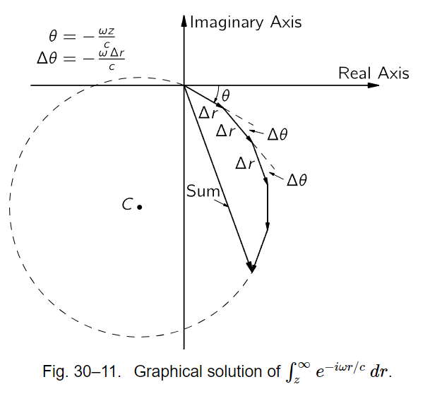
We can understand (30.15) as a sum of many small complex numbers, each of magnitude Δr, and with the angle θ=−ωr/c in the complex plane. We can try to evaluate the sum by a graphical method. In Fig. 30–11 we have drawn the first five pieces of the sum. Each segment of the curve has the length Δr and is placed at the angle Δθ=−ωΔr/c with respect to the preceding piece. The sum for these first five pieces is represented by the arrow from the starting point to the end of the fifth segment. As we continue to add pieces, we shall trace out a polygon until we get back to the starting point (approximately) and then start around once more. Adding more pieces, we just go round and round, staying close to a circle whose radius is easily shown to be c/ω. We can see now why the integral does not give a definite answer!
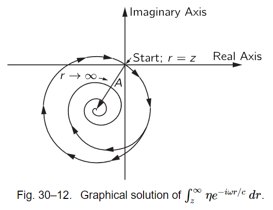
But now we have to go back to the physics of the situation. In any real situation the plane of charges cannot be infinite in extent, but must sometime stop. If it stopped suddenly, and was exactly circular in shape, our integral would have some value on the circle in Fig. 30–11. If, however, we let the number of charges in the plane gradually taper off at some large distance from the center (or else stop suddenly but in an irregular shape so for larger ρ the entire ring of width dρ no longer contributes), then the coefficient η in the exact integral would decrease toward zero. Since we are adding smaller pieces but still turning through the same angle, the graph of our integral would then become a curve which is a spiral. The spiral would eventually end up at the center of our original circle, as drawn in Fig. 30–12. The physically correct integral is the complex number A in the figure represented by the interval from the starting point to the center of the circle, which is just equal to
as you can work out for yourself. This is the same result we would get from Eq. (30.16) if we set e−i∞=0.
(There is also another reason why the contribution to the integral tapers off for large values of r, and that is the factor we have omitted for the projection of the acceleration on the plane perpendicular to the line PQ.)
We are, of course, interested only in physical situations, so we will take e−i∞ equal to zero. Returning to our original formula (30.12) for the field and putting back all of the factors that go with the integral, we have the result
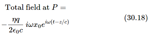
(Remembering that 1/i=−i).
It is interesting to note that (iωx0eiωt) is just equal to the velocity of the charges, so that we can also write the equation for the field as
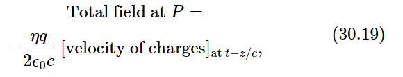
which is a little strange, because the retardation is just by the distance z, which is the shortest distance from P to the plane of charges. But that is the way it comes out—fortunately a rather simple formula. (We may add, by the way, that although our derivation is valid only for distances far from the plane of oscillatory charges, it turns out that the formula (30.18) or (30.19) is correct at any distance z, even for z<λ.)


|
|
|
|
دخلت غرفة فنسيت ماذا تريد من داخلها.. خبير يفسر الحالة
|
|
|
|
|
|
|
ثورة طبية.. ابتكار أصغر جهاز لتنظيم ضربات القلب في العالم
|
|
|
|
|
|
|
العتبة العباسية المقدسة تقدم دعوة إلى كلية مزايا الجامعة للمشاركة في حفل التخرج المركزي الخامس
|
|
|