Sample Variance Distribution

Let  samples be taken from a population with central moments . The sample variance  is then given by

(1)

where  is the sample mean.

The expected value of  for a sample size  is then given by

(2)

Similarly, the expected variance of the sample variance is given by

			(3)
			(4)

(Kenney and Keeping 1951, p. 164; Rose and Smith 2002, p. 264).

The algebra of deriving equation (4) by hand is rather tedious, but can be performed as follows. Begin by noting that

(5)

so

(6)

The value of  is already known from equation (◇), so it remains only to find . The algebra is simplified considerably by immediately transforming variables to  and performing computations with respect to these central variables. Since the variance does not depend on the mean  of the underlying distribution, the result obtained using the transformed variables will give an identical result while immediately eliminating expectation values of sums of terms containing odd powers of  (which equal 0). To determine , expand equation (6) to obtain

			(7)
			(8)
			(9)
			(10)

Working on the first term of (10),

			(11)
			(12)
			(13)
			(14)

The second term of (◇) is given by

			(15)
			(16)

and the third term by

			(17)
			(18)
			(19)

Plugging (◇)-(19) into (◇) then gives

			(20)
			(21)
			(22)
			(23)

(Kenney and Keeping 1951, p. 164). Plugging (◇) and (23) into (◇) then gives

			(24)
			(25)

as before.

For a normal distribution,  and , so

			(26)
			(27)

The third ane fourth moments of  are given by

			(28)
			(29)

giving the skewness and kurtosis excess of the distribution of the  as

			(30)
			(31)

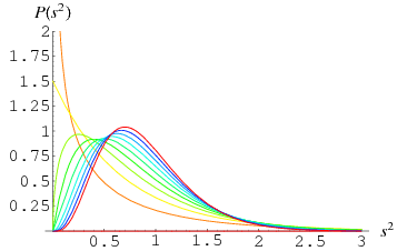
as computed by Student. Student also conjectured that the underlying distribution is Pearson type III distribution

(32)

where  is the gamma function--a conjecture that was subsequently proven by R. A. Fisher. Curves are illustrated above for  and  varying from  to 10.

REFERENCES:

Kenney, J. F. and Keeping, E. S. Mathematics of Statistics, Pt. 2, 2nd ed. Princeton, NJ: Van Nostrand, 1951.

Rose, C. and Smith, M. D. Mathematical Statistics with Mathematica. New York: Springer-Verlag, 2002.