آخر المواضيع المضافة

 تاريخ الرياضيات
الرياضيات في الحضارات المختلفة
الرياضيات المتقطعة
الجبر
الهندسة
المعادلات التفاضلية و التكاملية
التحليل
علماء الرياضيات
تاريخ الرياضيات
الرياضيات في الحضارات المختلفة
الرياضيات المتقطعة
الجبر
الهندسة
المعادلات التفاضلية و التكاملية
التحليل
علماء الرياضيات | Directed Graphs-Acyclic digraphs |


|
|
Read More
Date: 10-4-2022
Date: 13-3-2022
Date: 1-3-2022
|
Acyclic digraphs
Digraphs without circuits, or acyclic digraphs, have important applications, notably in scheduling with the potential task graph (defined in Chapter of Optimal Paths). We will give below one very useful characteristic property of these digraphs.
In general, a source of a digraph is a vertex with a zero indegree, that is a vertex without entering arcs. Likewise, a sink is a vertex with a zero outdegree, that is a vertex without exiting arcs.
Lemma 1.1. In a digraph without circuits, there are a source and a sink.
Proof. Consider any vertex x1, then, if it exists, a predecessor x2 of x1 and a predecessor x3 of x2, and so on as long as a predecessor to the vertex under consideration can be found. This construction of a sequence of vertices necessarily stops after a finite number of vertices. Indeed, the digraph being finite and having by hypothesis no circuit, it is not possible to encounter a vertex seen previously again. When this construction stops, we have a vertex which by construction has no predecessor, that is we obtain a source of the digraph, the existence of which is thus proven. It is possible to proceed likewise for a sink (or to consider the converse, that is, the digraph obtained by reversing the direction of the arcs: a source vertex of one is a sink vertex of the other).
Acyclic numbering
An acyclic numbering of the vertices of a digraph G =(X,A)is a bijection f from X onto the interval of integers from 1 to n (n is the number of vertices of G), such that if the ordered pair (x, y)is associated withan arc of G, then f(x) <f(y). The digraph is considered to be connected (underlying graph) and strict.
Proposition 1.1. A digraph G is without circuits if and only if it allows an acyclic numbering of its vertices.
Proof. The sufficient condition is easy to verify. Indeed, if there were a circuit defined by the sequence of its vertices (x0,x1,...,x0), we would have f(x0) < f(x1) < ··· <f(x0) and therefore a contradiction since then f(x0) <f(x0). For the necessary condition we can consider a source vertex x1 of G (which we know exists from lemma 1.1) and put f(x1) = 1, then continue with digraph G1 = G − x1 in place of G, that is consider a source vertex x2 of G1 for which we put f(x2)=2.Weremove x2 from G1 and start again with G2 = G1 −x2 in place of G1, and so on, while there is at least one vertex left in the current digraph. Note that each of the graphs successively considered, G1,G2,..., is really without circuits, as it is a subdigraph of G. It is easy to verify that, by construction, the application f thus defined is an acyclic numbering of the vertices of G.
Note. The algorithmic aspect of the construction of acyclic numbering is in practice very important. The preceding proof does give an algorithm but one which is not very good from an implementation and complexity viewpoint. Indeed, the removal of the vertex in the digraph complicates things. We will see a much better algorithm later, using a depth-first search of the digraph
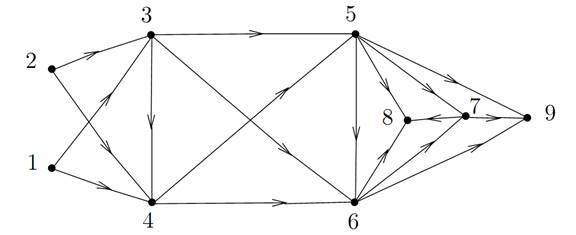
Figure 1.1. A digraph without circuits with its vertices numbered according to an acyclic numbering. The vertices 1 and 2 are source, the vertices 8 and 9aresink
Practical aspects
In practice, we use a concept close to acyclic numbering of vertices,which is a classification of the vertices by levels. The important property is then that at each level a vertex has only predecessors at lower levels. We have a similar property to acyclic numbering, but the acyclic numbering is more directly usable since we always end uplooking at the vertices in a certain order. Let us therefore remember whatis most essential here, which is how we will apply it all later on: when we consider the vertices of a digraph in the order of an acyclic numbering, atthe time when a given vertex is considered, all its predecessors have been considered. Thus, if we have to apply a certain treatment on each vertex ofa digraph without circuits, and this treatment uses the result of this same treatment on the predecessors of the vertex under consideration, then thistreatment done in the order of an acyclic numbering will be possible on all the vertices of the digraph.
Arborescences
The root of a digraph G is a vertex r such that there is for any vertex x of G a directed path from r to x.
An arborescence is a digraph which has a root and of which the underlying graph is a tree. In the literature, the term tree is often used instead of arborescence.
Note. An arborescence has only one root (but generally speaking, a digraph may have several roots).
Drawings
We usually draw an arborescence with the root at the top (which would make us say that here the trees have their roots up in the air!), and the other vertices arranged horizontally by levels of equal distances from the root. The arrows indicating the orientation of the arcs are occasionally omitted as they are implicitly defined as going from top to bottom (see Figure 1.2).

Figure 1.2. Different drawings of an arborescence
Note. An arborescence is identified by a (undirected) tree with a distinguished vertex called the root. The orientation of the arcs may be found by following the direction of the increasing distance from this root on each edge. (Note that this direction is uniquely defined because of the uniqueness of the directed path from the root to a vertex in an arborescence, according to a property given later on.) That is why arborescences are often called rooted trees in the literature, or simply trees.
Terminology
An arborescence, as for any digraph without circuits, has at least one sink and usually there are many. Such a vertex is called a leaf. In general the vertices of an arborescence are called nodes. The depth of a vertex is its distance from the root (“distance” heremeans the shortest lengthof the directed paths). This term refers to the usual drawing of arborescences, in which, as we saw, the vertices with thesame depth are placed on what is called a same depth level.
The depth of an arborescence is the greatest depth of its vertex.
Terminology inspired by that of genealogical trees can also be used. A child of a vertex is any successor to that vertex. A vertex without a child is a leaf. If vertex y is a child of vertex x, x is then naturally called the parent of y. Any vertex of an arborescence has a unique parent except for the root, which has none. Vertices which share the same parent are then also very naturally called siblings. This terminology – parent, child, sibling – is useful for “surfing” in an arborescence as we will see in the following chapter. More generally, a descendant of a vertex x of an arborescence is the name given to any vertex y such that there is in the arborescence a directed path going from x to y. In other words, y is a successor or, in a repeated fashion, a successor of a successor of x.
Characterization of arborescences
Theorem 1.1. For a digraph G, the following conditions are equivalent:
(1) G is an arborescence.
(2) G has a root and its underlying graph is acyclic.
(3) G has a root and m = n − 1.
(4) There is a vertex r such that for any vertex x of G there is a unique directed path going from r to x.
(5) G is connected and d−(x)=1 for any vertex x except for one vertex, r, for which d−(r)=0. (This last condition will be referred to below as the “indegrees condition”.)
(6) The underlying graph of G is acyclic and we have the property of the indegrees condition.
(7) G has no circuits and we have the indegrees condition.
Proof (sketch). Let us give a “complete” set of implications, complete in the sense that any other implication may be deduced from it by transitivity (we apply here a concept of “transitive closure”,). The implications to verify, chosen for their ease, are:
– equivalence of conditions (1), (2), and (3);
– equivalence of (6) and (7);
–(1)⇒(4), (4)⇒(5), (5)⇒(6), (6)⇒(1).
Note. In condition (4), the unique directed path from vertex r to itself is the directed path with of zero length and unique vertex r.
Subarborescences
Given an arborescence T and one of its vertices s, the subarborescence of root s is the subdigraph of T induced by s and all its descendants in T.
This subdigraph is an arborescence, with vertex s for its root.
Ordered arborescences
It is frequent in applications to consider what can be called an ordered arborescence, that is an arborescence in which an (total) order is given to the set of the children of each vertex. In general, this is the case in practice since an arborescence is often defined for each vertex by the data of its children in a list, that is with a certain order. In the case of an ordered arborescence, it is possible to speak of the first child or of the following sibling of a vertex (as we will do, for example, in the following chapter).
Looking at the arborescence in Figure 1.2, and more specifically the bottom drawings representing an ordered arborescence (from left to right for the children of each vertex), we see for example that: d is the first child of b, e is the following sibling of d, e has no following sibling.
Directed forests
A directed forest is a digraph in which each connected component is an arborescence. The underlying graph is of course a forest, and a directed forest can be identified with a forest in which each connected component has a distinct vertex which is its root. The properties of directed forests can be deduced from those of the arborescences applied to its components.
Graph Theory and Applications ,Jean-Claude Fournier, WILEY, page(90-95)
|
|
|
|
تفوقت في الاختبار على الجميع.. فاكهة "خارقة" في عالم التغذية
|
|
|
|
|
|
|
أمين عام أوبك: النفط الخام والغاز الطبيعي "هبة من الله"
|
|
|
|
|
|
|
المجمع العلمي ينظّم ندوة حوارية حول مفهوم العولمة الرقمية في بابل
|
|
|