آخر المواضيع المضافة

 الفيزياء الكلاسيكية
الكهربائية والمغناطيسية
علم البصريات
الفيزياء الحديثة
النظرية النسبية
الفيزياء النووية
فيزياء الحالة الصلبة
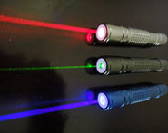
الليزر
علم الفلك
المجموعة الشمسية
الطاقة البديلة
الفيزياء والعلوم الأخرى
مواضيع عامة في الفيزياء
الفيزياء الكلاسيكية
الكهربائية والمغناطيسية
علم البصريات
الفيزياء الحديثة
النظرية النسبية
الفيزياء النووية
فيزياء الحالة الصلبة
الليزر
علم الفلك
المجموعة الشمسية
الطاقة البديلة
الفيزياء والعلوم الأخرى
مواضيع عامة في الفيزياء| Resonance in nature |


|
|
أقرأ أيضاً
التاريخ: 21-1-2016
التاريخ: 1-1-2017
التاريخ: 4-12-2020
التاريخ: 28-2-2016
|
We could bring up case after case in many fields, and show exactly how the resonance equation is the same. There are many circumstances in nature in which something is “oscillating” and in which the resonance phenomenon occurs. We said that in an earlier chapter; let us now demonstrate it. If we walk around our study, pulling books off the shelves and simply looking through them to find an example of a curve that corresponds to Fig. 23–2 and comes from the same equation, what do we find? Just to demonstrate the wide range obtained by taking the smallest possible sample, it takes only five or six books to produce quite a series of phenomena which show resonances.
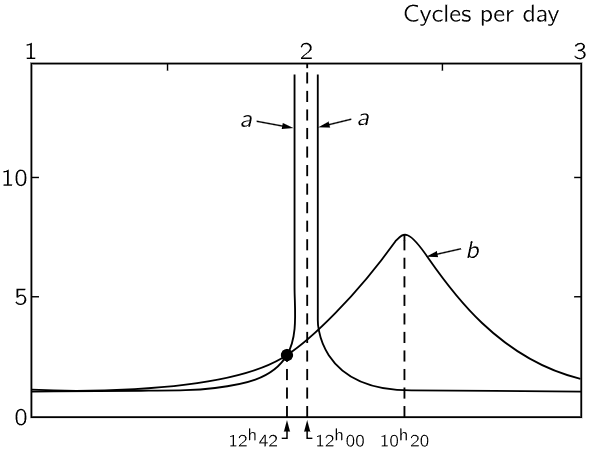
Fig. 23–6. Response of the atmosphere to external excitation. a is the required response if the atmospheric S2-tide is of gravitational origin; peak amplification is 100:1. b is derived from observed magnification and phase of M2-tide. [Munk and MacDonald, “Rotation of the Earth,” Cambridge University Press (1960)]
The first two are from mechanics, the first on a large scale: the atmosphere of the whole earth. If the atmosphere, which we suppose surrounds the earth evenly on all sides, is pulled to one side by the moon or, rather, squashed prolate into a double tide, and if we could then let it go, it would go sloshing up and down; it is an oscillator. This oscillator is driven by the moon, which is effectively revolving about the earth; any one component of the force, say in the x-direction, has a cosine component, and so the response of the earth’s atmosphere to the tidal pull of the moon is that of an oscillator. The expected response of the atmosphere is shown in Fig. 23–6, curve b (curve a is another theoretical curve under discussion in the book from which this is taken out of context). Now one might think that we only have one point on this resonance curve, since we only have the one frequency, corresponding to the rotation of the earth under the moon, which occurs at a period of 12.42 hours—12 hours for the earth (the tide is a double bump), plus a little more because the moon is going around. But from the size of the atmospheric tides, and from the phase, the amount of delay, we can get both ρ and θ. From those we can get ω0 and γ, and thus draw the entire curve! This is an example of very poor science. From two numbers we obtain two numbers, and from those two numbers we draw a beautiful curve, which of course goes through the very point that determined the curve! It is of no use unless we can measure something else, and in the case of geophysics that is often very difficult. But in this particular case there is another thing which we can show theoretically must have the same timing as the natural frequency ω0: that is, if someone disturbed the atmosphere, it would oscillate with the frequency ω0. Now there was such a sharp disturbance in 1883; the Krakatoa volcano exploded and half the island blew off, and it made such a terrific explosion in the atmosphere that the period of oscillation of the atmosphere could be measured. It came out to 10 1/2 hours. The ω0 obtained from Fig. 23–6 comes out 10 hours and 20 minutes, so there we have at least one check on the reality of our understanding of the atmospheric tides.
Next we go to the small scale of mechanical oscillation. This time we take a sodium chloride crystal, which has sodium ions and chlorine ions next to each other, as we described in an early chapter. These ions are electrically charged, alternately plus and minus. Now there is an interesting oscillation possible. Suppose that we could drive all the plus charges to the right and all the negative charges to the left, and let go; they would then oscillate back and forth, the sodium lattice against the chlorine lattice. How can we ever drive such a thing? That is easy, for if we apply an electric field on the crystal, it will push the plus charge one way and the minus charge the other way! So, by having an external electric field we can perhaps get the crystal to oscillate. The frequency of the electric field needed is so high, however, that it corresponds to infrared radiation! So, we try to find a resonance curve by measuring the absorption of infrared light by sodium chloride. Such a curve is shown in Fig. 23–7. The abscissa is not frequency, but is given in terms of wavelength, but that is just a technical matter, of course, since for a wave there is a definite relation between frequency and wavelength; so, it is really a frequency scale, and a certain frequency corresponds to the resonant frequency.
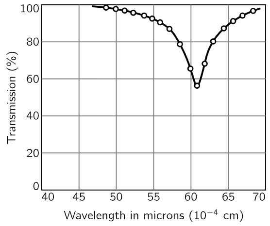
Fig. 23–7. Transmission of infrared radiation through a thin (0.17 μm) sodium chloride film. [After R. B. Barnes, Z. Physik 75, 723 (1932). Kittel, Introduction to Solid State Physics, Wiley, 1956.]
But what about the width? What determines the width? There are many cases in which the width that is seen on the curve is not really the natural width γ that one would have theoretically. There are two reasons why there can be a wider curve than the theoretical curve. If the objects do not all have the same frequency, as might happen if the crystal were strained in certain regions, so that in those regions the oscillation frequency were slightly different than in other regions, then what we have is many resonance curves on top of each other; so we apparently get a wider curve. The other kind of width is simply this: perhaps we cannot measure the frequency precisely enough—if we open the slit of the spectrometer fairly wide, so although we thought we had only one frequency, we actually had a certain range Δω, then we may not have the resolving power needed to see a narrow curve. Offhand, we cannot say whether the width in Fig. 23–7 is natural, or whether it is due to inhomogeneities in the crystal or the finite width of the slit of the spectrometer.
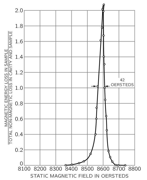
Fig. 23–8. Magnetic energy loss in paramagnetic organic compound as function of applied magnetic field intensity. [Holden et al., Phys. Rev. 75, 1614 (1949)]
Now we turn to a more esoteric example, and that is the swinging of a magnet. If we have a magnet, with north and south poles, in a constant magnetic field, the N end of the magnet will be pulled one way and the S end the other way, and there will in general be a torque on it, so it will vibrate about its equilibrium position, like a compass needle. However, the magnets we are talking about are atoms. These atoms have an angular momentum, the torque does not produce a simple motion in the direction of the field, but instead, of course, a precession. Now, looked at from the side, any one component is “swinging,” and we can disturb or drive that swinging and measure an absorption. The curve in Fig. 23–8 represents a typical such resonance curve. What has been done here is slightly different technically. The frequency of the lateral field that is used to drive this swinging is always kept the same, while we would have expected that the investigators would vary that and plot the curve. They could have done it that way, but technically it was easier for them to leave the frequency ω fixed, and change the strength of the constant magnetic field, which corresponds to changing ω0 in our formula. They have plotted the resonance curve against ω0. Anyway, this is a typical resonance with a certain ω0 and γ.
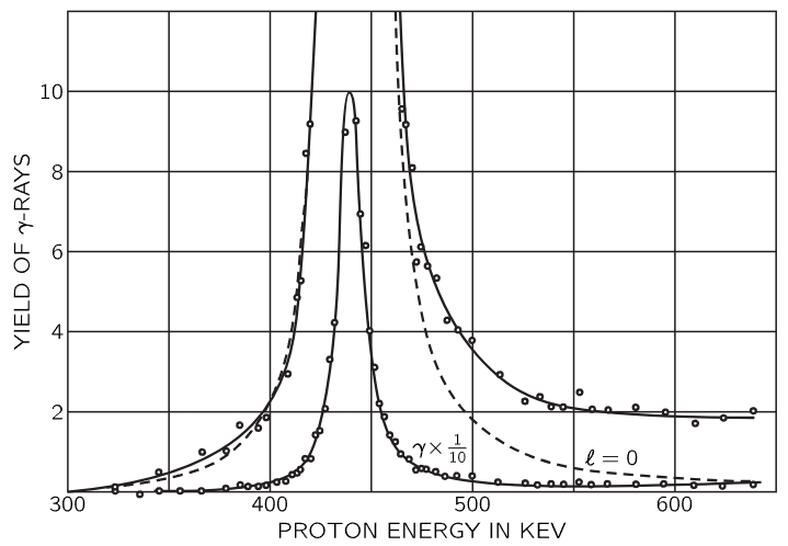
Fig. 23–9. The intensity of gamma-radiation from lithium as a function of the energy of the bombarding protons. The dashed curve is a theoretical one calculated for protons with an angular momentum ℓ=0. [Bonner and Evans, Phys. Rev. 73, 666 (1948)]
Now we go still further. Our next example has to do with atomic nuclei. The motions of protons and neutrons in nuclei are oscillatory in certain ways, and we can demonstrate this by the following experiment. We bombard a lithium atom with protons, and we discover that a certain reaction, producing γ-rays, actually has a very sharp maximum typical of resonance. We note in Fig. 23–9, however, one difference from other cases: the horizontal scale is not a frequency, it is an energy! The reason is that in quantum mechanics what we think of classically as the energy will turn out to be really related to a frequency of a wave amplitude. When we analyze something which in simple large-scale physics has to do with a frequency, we find that when we do quantum-mechanical experiments with atomic matter, we get the corresponding curve as a function of energy. In fact, this curve is a demonstration of this relationship, in a sense. It shows that frequency and energy have some deep interrelationship, which of course they do.
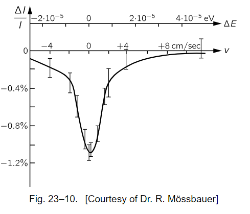
Now we turn to another example which also involves a nuclear energy level, but now a much, much narrower one. The ω0 in Fig. 23–10 corresponds to an energy of 100,000 electron volts, while the width γ is approximately 10−5 electron volt; in other words, this has a Q of 1010! When this curve was measured it was the largest Q of any oscillator that had ever been measured. It was measured by Dr. Mössbauer, and it was the basis of his Nobel prize. The horizontal scale here is velocity, because the technique for obtaining the slightly different frequencies was to use the Doppler effect, by moving the source relative to the absorber. One can see how delicate the experiment is when we realize that the speed involved is a few centimeters per second! On the actual scale of the figure, zero frequency would correspond to a point about 1010 cm to the left—slightly off the paper!
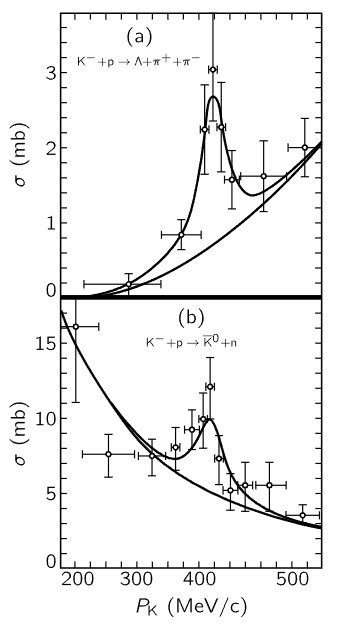
Fig. 23–11. Momentum dependence of the cross section for the reactions (a) K−+p→Λ+π++π− and (b) K−+p→K¯0+n. The lower curves in (a) and (b) represent the presumed nonresonant backgrounds, while the upper curves contain in addition the superposed resonance. [Ferro-Luzzi et al., Phys. Rev. Lett. 8, 28 (1962)]
Finally, if we look in an issue of the Physical Review, say that of January 1, 1962, will we find a resonance curve? Every issue has a resonance curve, and Fig. 23–11 is the resonance curve for this one. This resonance curve turns out to be very interesting. It is the resonance found in a certain reaction among strange particles, a reaction in which a K− and a proton interact. The resonance is detected by seeing how many of some kinds of particles come out, and depending on what and how many come out, one gets different curves, but of the same shape and with the peak at the same energy. We thus determine that there is a resonance at a certain energy for the K− meson. That presumably means that there is some kind of a state, or condition, corresponding to this resonance, which can be attained by putting together a K− and a proton. This is a new particle, or resonance. Today we do not know whether to call a bump like this a “particle” or simply a resonance. When there is a very sharp resonance, it corresponds to a very definite energy, just as though there were a particle of that energy present in nature. When the resonance gets wider, then we do not know whether to say there is a particle which does not last very long, or simply a resonance in the reaction probability.


|
|
|
|
هل يمكن للدماغ البشري التنبؤ بالمستقبل أثناء النوم؟
|
|
|
|
|
|
|
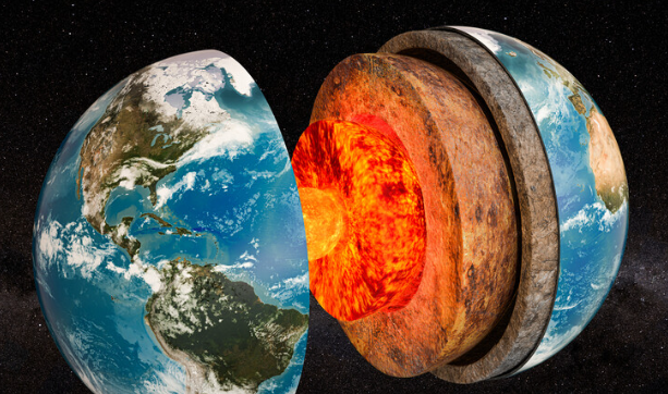
علماء: طول الأيام على الأرض يزداد بسبب النواة الداخلية
|
|
|
|
|
|
|
المجمع العلمي يحيي زيارة يوم عرفة
|
|
|