The difficulty above was another part of the continual problem of classical physics, which started with the difficulty of the specific heat of gases, and now has been focused on the distribution of light in a blackbody. Now, of course, at the time that theoreticians studied this thing, there were also many measurements of the actual curve. And it turned out that the correct curve looked like the dashed curves in Fig. 41–4.

Fig. 41–4. The blackbody intensity distribution at two temperatures, according to classical physics (solid curves). The dashed curves show the actual distribution.

That is, the x-rays were not there. If we lower the temperature, the whole curve goes down in proportion to T, according to the classical theory, but the observed curve also cuts off sooner at a lower temperature. Thus, the low-frequency end of the curve is right, but the high-frequency end is wrong. Why? When Sir James Jeans was worrying about the specific heats of gases, he noted that motions which have high frequency are “frozen out” as the temperature goes too low. That is, if the temperature is too low, if the frequency is too high, the oscillators do not have kT of energy on the average. Now recall how our derivation of (41.13) worked: It all depends on the energy of an oscillator at thermal equilibrium. What the kT of (41.5) was, and what the same kT in (41.13) is, is the mean energy of a harmonic oscillator of frequency ω at temperature T.

Classically, this is kT, but experimentally, no! —not when the temperature is too low or the oscillator frequency is too high. And so, the reason that the curve falls off is the same reason that the specific heats of gases fail. It is easier to study the blackbody curve than it is the specific heats of gases, which are so complicated, therefore our attention is focused on determining the true blackbody curve, because this curve is a curve which correctly tells us, at every frequency, what the average energy of harmonic oscillators actually is as a function of temperature.

Planck studied this curve. He first determined the answer empirically, by fitting the observed curve with a nice function that fitted very well. Thus he had an empirical formula for the average energy of a harmonic oscillator as a function of frequency. In other words, he had the right formula instead of kT, and then by fiddling around he found a simple derivation for it which involved a very peculiar assumption. That assumption was that the harmonic oscillator can take up energies only ℏω at a time. The idea that they can have any energy at all is false. Of course, that was the beginning of the end of classical mechanics.

Fig. 41–5. The energy levels of a harmonic oscillator are equally spaced: E_n=nℏω.

The very first correctly determined quantum-mechanical formula will now be derived. Suppose that the permitted energy levels of a harmonic oscillator were equally spaced at ℏω₀ apart, so that the oscillator could take on only these different energies (Fig. 41–5). Planck made a somewhat more complicated argument than the one that is being given here, because that was the very beginning of quantum mechanics and he had to prove some things. But we are going to take it as a fact (which he demonstrated in this case) that the probability of occupying a level of energy E is P(E)=αe^−E/kT. If we go along with that, we will obtain the right result.

Suppose now that we have a lot of oscillators, and each is a vibrator of frequency ω₀. Some of these vibrators will be in the bottom quantum state, some will be in the next one, and so forth. What we would like to know is the average energy of all these oscillators. To find out, let us calculate the total energy of all the oscillators and divide by the number of oscillators. That will be the average energy per oscillator in thermal equilibrium, and will also be the energy that is in equilibrium with the blackbody radiation and that should go in Eq. (41.13) in place of kT. Thus, we let N₀ be the number of oscillators that are in the ground state (the lowest energy state); N₁ the number of oscillators in the state E₁; N₂ the number that are in state E₂; and so on. According to the hypothesis (which we have not proved) that in quantum mechanics the law that replaced the probability e^−P.E./kT or e^−K.E./kT in classical mechanics is that the probability goes down as e^−ΔE/kT, where ΔE is the excess energy, we shall assume that the number N₁ that are in the first state will be the number N₀ that are in the ground state, times e^−ℏω/kT. Similarly, N₂, the number of oscillators in the second state, is N₂=N₀e^−2ℏω/kT. To simplify the algebra, let us call e^−ℏω/kT=x. Then we simply have N₁=N₀x, N₂=N₀x², …, N_n=N₀xⁿ.

The total energy of all the oscillators must first be worked out. If an oscillator is in the ground state, there is no energy. If it is in the first state, the energy is ℏω, and there are N₁ of them. So N₁ℏω, or ℏωN₀x is how much energy we get from those. Those that are in the second state have 2ℏω, and there are N₂ of them, so N₂⋅2ℏω=2ℏωN₀x² is how much energy we get, and so on. Then we add it all together to get E_tot=N₀ℏω(0+x+2x²+3x³+⋯).

And now, how many oscillators are there? Of course, N₀ is the number that are in the ground state, N₁ in the first state, and so on, and we add them together: N_tot=N₀(1+x+x²+x³+⋯). Thus the average energy is

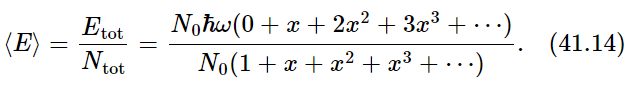
Now the two sums which appear here we shall leave for the reader to play with and have some fun with. When we are all finished summing and substituting for x in the sum, we should get—if we make no mistakes in the sum—

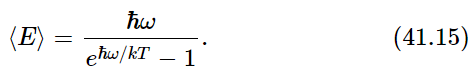
This, then, was the first quantum-mechanical formula ever known, or ever discussed, and it was the beautiful culmination of decades of puzzlement. Maxwell knew that there was something wrong, and the problem was, what was right? Here is the quantitative answer of what is right instead of kT. This expression should, of course, approach kT as ω→0 or as T→∞. See if you can prove that it does—learn how to do the mathematics.

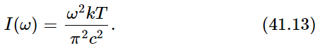
This is the famous cutoff factor that Jeans was looking for, and if we use it instead of kT in (41.13), we obtain for the distribution of light in a black box

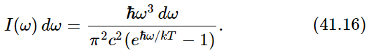
We see that for a large ω, even though we have ω³ in the numerator, there is an e raised to a tremendous power in the denominator, so the curve comes down again and does not “blow up”—we do not get ultraviolet light and x-rays where we do not expect them!

One might complain that in our derivation of (41.16) we used the quantum theory for the energy levels of the harmonic oscillator, but the classical theory in determining the cross section σ_s. But the quantum theory of light interacting with a harmonic oscillator gives exactly the same result as that given by the classical theory. That, in fact, is why we were justified in spending so much time on our analysis of the index of refraction and the scattering of light, using a model of atoms like little oscillators—the quantum formulas are substantially the same.

Now let us return to the Johnson noise in a resistor. We have already remarked that the theory of this noise power is really the same theory as that of the classical blackbody distribution. In fact, rather amusingly, we have already said that if the resistance in a circuit were not a real resistance, but were an antenna (an antenna acts like a resistance because it radiates energy), a radiation resistance, it would be easy for us to calculate what the power would be. It would be just the power that runs into the antenna from the light that is all around, and we would get the same distribution, changed by only one or two factors. We can suppose that the resistor is a generator with an unknown power spectrum P(ω). The spectrum is determined by the fact that this same generator, connected to a resonant circuit of any frequency, as in Fig. 41–2(b), generates in the inductance a voltage of the magnitude given in Eq. (41.2).

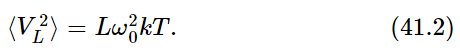
Fig. 41–2.A high-Q resonant circuit. (a) Actual circuit, at temperature T. (b) Artificial circuit, with an ideal (noiseless) resistance and a “noise generator” G.

One is thus led to the same integral as in (41.10), and the same method works to give Eq. (41.3). For low temperatures the kT in (41.3) must of course be replaced by (41.15). The two theories (blackbody radiation and Johnson noise) are also closely related physically, for we may of course connect a resonant circuit to an antenna, so the resistance R is a pure radiation resistance. Since (41.2) does not depend on the physical origin of the resistance, we know the generator G for a real resistance and for radiation resistance is the same.

What is the origin of the generated power P(ω) if the resistance R is only an ideal antenna in equilibrium with its environment at temperature T? It is the radiation I(ω) in the space at temperature T which impinges on the antenna and, as “received signals,” makes an effective generator.

All the things we have been talking about—the so-called Johnson noise and Planck’s distribution, and the correct theory of the Brownian movement which we are about to describe—are developments of the first decade or so of the 20th century. Now with those points and that history in mind, we return to the Brownian movement.

مواضيع ذات صلة

philosophical implications of quantum mechanics

Crystal diffraction

Measurement of position and momentum

Probability wave amplitudes

The uncertainty principle

First principles of quantum mechanics

Watching the electrons

An experiment with electrons

An experiment with waves

An experiment with bullets

Chance and likelihood

Short distances