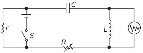
Fig. 24–2. An electrical circuit for demonstrating transients.

Now let us see if the above really works. We construct the electrical circuit shown in Fig. 24–2, in which we apply to an oscilloscope the voltage across the inductance L after we suddenly turn on a voltage by closing the switch S. It is an oscillatory circuit, and it generates a transient of some kind. It corresponds to a circumstance in which we suddenly apply a force and the system starts to oscillate. It is the electrical analog of a damped mechanical oscillator, and we watch the oscillation on an oscilloscope, where we should see the curves that we were trying to analyze. (The horizontal motion of the oscilloscope is driven at a uniform speed, while the vertical motion is the voltage across the inductor. The rest of the circuit is only a technical detail. We would like to repeat the experiment many, many times, since the persistence of vision is not good enough to see only one trace on the screen. So, we do the experiment again and again by closing the switch 60 times a second; each time we close the switch, we also start the oscilloscope horizontal sweep, and it draws the curve over and over.) In Figs. 24–3 to 24–6 we see examples of damped oscillations, actually photographed on an oscilloscope screen. Figure 24–3 shows a damped oscillation in a circuit which has a high Q, a small γ. It does not die out very fast; it oscillates many times on the way down.

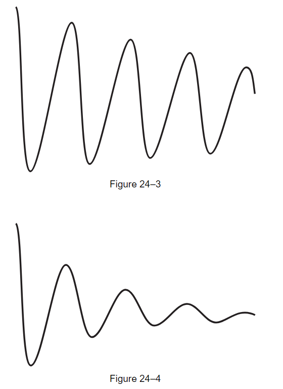
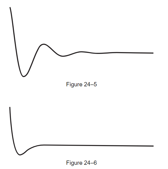
But let us see what happens as we decrease Q, so that the oscillation dies out more rapidly. We can decrease Q by increasing the resistance R in the circuit. When we increase the resistance in the circuit, it dies out faster (Fig. 24–4). Then if we increase the resistance in the circuit still more, it dies out faster still (Fig. 24–5). But when we put in more than a certain amount, we cannot see any oscillation at all! The question is, is this because our eyes are not good enough? If we increase the resistance still more, we get a curve like that of Fig. 24–6, which does not appear to have any oscillations, except perhaps one. Now, how can we explain that by mathematics?

The resistance is, of course, proportional to the γ term in the mechanical device. Specifically, γ is R/L. Now if we increase the γ in the solutions (24.14) and (24.15) that we were so happy with before, chaos sets in when γ/2 exceeds ω₀; we must write it a different way, as

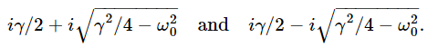
Those are now the two solutions and, following the same line of mathematical reasoning as previously, we again find two solutions: e^iα₁t and e^iα₂t. If we now substitute for α₁, we get

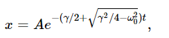
a nice exponential decay with no oscillations. Likewise, the other solution is

Note that the square root cannot exceed γ/2, because even if ω₀=0, one term just equals the other. But ω²₀ is taken away from γ²/4, so the square root is less than γ/2, and the term in parentheses is, therefore, always a positive number. Thank goodness! Why? Because if it were negative, we would find e raised to a positive factor times t, which would mean it was exploding! In putting more and more resistance into the circuit, we know it is not going to explode—quite the contrary. So now we have two solutions, each one by itself a dying exponential, but one having a much faster “dying rate” than the other. The general solution is of course a combination of the two; the coefficients in the combination depending upon how the motion starts—what the initial conditions of the problem are. In the particular way this circuit happens to be starting, the A is negative and the B is positive, so we get the difference of two exponential curves.

Now let us discuss how we can find the two coefficients A and B (or A and A^∗), if we know how the motion was started.

Suppose that at t=0 we know that x=x₀, and dx/dt=v₀. If we put t=0, x=x₀, and dx/dt=v₀ into the expressions

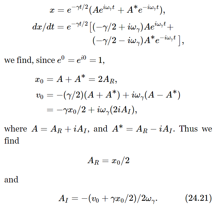
This completely determines A and A^∗, and therefore the complete curve of the transient solution, in terms of how it begins. Incidentally, we can write the solution another way if we note that

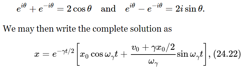
Where 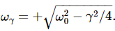. This is the mathematical expression for the way an oscillation dies out. We shall not make direct use of it, but there are a number of points we should like to emphasize that are true in more general cases.

First of all the behavior of such a system with no external force is expressed by a sum, or superposition, of pure exponentials in time (which we wrote as e^iαt). This is a good solution to try in such circumstances. The values of α may be complex in general, the imaginary parts representing damping. Finally, the intimate mathematical relation of the sinusoidal and exponential function often appears physically as a change from oscillatory to exponential behavior when some physical parameter (in this case resistance, γ) exceeds some critical value.

مواضيع ذات صلة

الشرر المقدس

الحقول الكهربية والشرر

الخلق غير المرئي

عجائب الكهرباء

مصادر الطاقة الكهربائية

التيارات الكهربائية التي تجري إلى الابد

النقل الكهربائي وقانون أوم

مبردات الهواء

طرق التبريد

تأريض نقطة التعامل خلال ملف (النظام المؤرض بالرنين)

التأريض خلال ممانعة

مميزات نظام التأريض خلال مقاومة