0
settings
الوضع الليلي
moon
انماط الصفحة الرئيسية arrow
EN
1
المرجع الالكتروني للمعلوماتية

تاريخ الرياضيات

الاعداد و نظريتها

تاريخ التحليل

تار يخ الجبر

الهندسة و التبلوجي

الرياضيات في الحضارات المختلفة

العربية

اليونانية

البابلية

الصينية

المايا

المصرية

الهندية

الرياضيات المتقطعة

المنطق

اسس الرياضيات

فلسفة الرياضيات

مواضيع عامة في المنطق

الجبر

الجبر الخطي

الجبر المجرد

الجبر البولياني

مواضيع عامة في الجبر

الضبابية

نظرية المجموعات

نظرية الزمر

نظرية الحلقات والحقول

نظرية الاعداد

نظرية الفئات

حساب المتجهات

المتتاليات-المتسلسلات

المصفوفات و نظريتها

المثلثات

الهندسة

الهندسة المستوية

الهندسة غير المستوية

مواضيع عامة في الهندسة

التفاضل و التكامل

المعادلات التفاضلية و التكاملية

معادلات تفاضلية

معادلات تكاملية

مواضيع عامة في المعادلات

التحليل

التحليل العددي

التحليل العقدي

التحليل الدالي

مواضيع عامة في التحليل

التحليل الحقيقي

التبلوجيا

نظرية الالعاب

الاحتمالات و الاحصاء

نظرية التحكم

بحوث العمليات

نظرية الكم

الشفرات

الرياضيات التطبيقية

نظريات ومبرهنات

علماء الرياضيات

500AD

500-1499

1000to1499

1500to1599

1600to1649

1650to1699

1700to1749

1750to1779

1780to1799

1800to1819

1820to1829

1830to1839

1840to1849

1850to1859

1860to1864

1865to1869

1870to1874

1875to1879

1880to1884

1885to1889

1890to1894

1895to1899

1900to1904

1905to1909

1910to1914

1915to1919

1920to1924

1925to1929

1930to1939

1940to the present

علماء الرياضيات

الرياضيات في العلوم الاخرى

بحوث و اطاريح جامعية

هل تعلم

طرائق التدريس

الرياضيات العامة

نظرية البيان

قم بتسجيل الدخول اولاً لكي يتسنى لك الاعجاب والتعليق.

Gamma Distribution

المؤلف:  Beyer, W. H.

المصدر:  CRC Standard Mathematical Tables, 28th ed. Boca Raton, FL: CRC Press

الجزء والصفحة:  ...

6-4-2021

2290

+

-

20

Gamma Distribution

GammaDistribution

A gamma distribution is a general type of statistical distribution that is related to the beta distribution and arises naturally in processes for which the waiting times between Poisson distributed events are relevant. Gamma distributions have two free parameters, labeled alpha and theta, a few of which are illustrated above.

Consider the distribution function D(x) of waiting times until the hth Poisson event given a Poisson distribution with a rate of change lambda,

D(x) = P(X<=x)

(1)

= 1-P(X>x)

(2)

= 1-sum_(k=0)^(h-1)((lambdax)^ke^(-lambdax))/(k!)

(3)

= 1-e^(-lambdax)sum_(k=0)^(h-1)((lambdax)^k)/(k!)

(4)

= 1-(Gamma(h,xlambda))/(Gamma(h))

(5)

for x in [0,infty), where Gamma(x) is a complete gamma function, and Gamma(a,x) an incomplete gamma function. With h an integer, this distribution is a special case known as the Erlang distribution.

The corresponding probability function P(x) of waiting times until the hth Poisson event is then obtained by differentiating D(x),

P(x) =

(6)

= lambdae^(-lambdax)sum_(k=0)^(h-1)((lambdax)^k)/(k!)-e^(-lambdax)sum_(k=0)^(h-1)(k(lambdax)^(k-1)lambda)/(k!)

(7)

= lambdae^(-lambdax)+lambdae^(-lambdax)sum_(k=1)^(h-1)((lambdax)^k)/(k!)-e^(-lambdax)sum_(k=1)^(h-1)(k(lambdax)^(k-1)lambda)/(k!)

(8)

= lambdae^(-lambdax)-lambdae^(-lambdax)sum_(k=1)^(h-1)[(k(lambdax)^(k-1))/(k!)-((lambdax)^k)/(k!)]

(9)

= lambdae^(-lambdax)<span style={1-sum_(k=1)^(h-1)[((lambdax)^(k-1))/((k-1)!)-((lambdax)^k)/(k!)]}" src="https://mathworld.wolfram.com/images/equations/GammaDistribution/Inline42.gif" style="height:47px; width:204px" />

(10)

= lambdae^(-lambdax)<span style={1-[1-((lambdax)^(h-1))/((h-1)!)]}" src="https://mathworld.wolfram.com/images/equations/GammaDistribution/Inline45.gif" style="height:42px; width:156px" />

(11)

= (lambda(lambdax)^(h-1))/((h-1)!)e^(-lambdax).

(12)

Now let alpha=h (not necessarily an integer) and define theta=1/lambda to be the time between changes. Then the above equation can be written
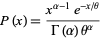
 P(x)=(x^(alpha-1)e^(-x/theta))/(Gamma(alpha)theta^alpha)

(13)

for x in [0,infty). This is the probability function for the gamma distribution, and the corresponding distribution function is
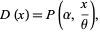
 D(x)=P(alpha,x/theta),

(14)

where P(a,z) is a regularized gamma function.

It is implemented in the Wolfram Language as the function GammaDistribution[alpha, theta].

The characteristic function describing this distribution is

phi(t) = F_x<span style={(x^(-x/theta)x^(alpha-1))/(Gamma(alpha)theta^alpha)[1/2(1+sgnx)]}(t)" src="https://mathworld.wolfram.com/images/equations/GammaDistribution/Inline55.gif" style="height:42px; width:192px" />

(15)

= (1-ittheta)^(-alpha),

(16)

where F_x[f](t) is the Fourier transform with parameters a=b=1, and the moment-generating function is

M(t) = int_0^infty(e^(tx)x^(alpha-1)e^(-x/theta)dx)/(Gamma(alpha)theta^alpha)

(17)

= int_0^infty(x^(alpha-1)e^(-(1-thetat)x/theta)dx)/(Gamma(alpha)theta^alpha).

(18)

giving moments about 0 of

(19)

(Papoulis 1984, p. 147).

In order to explicitly find the moments of the distribution using the moment-generating function, let

y = ((1-thetat)x)/theta

(20)

dy = (1-thetat)/thetadx,

(21)

so

M(t) = int_0^infty((thetay)/(1-thetat))^(alpha-1)(e^(-y))/(Gamma(alpha)theta^alpha)(thetady)/(1-thetat)

(22)

= 1/((1-thetat)^alphaGamma(alpha))int_0^inftyy^(alpha-1)e^(-y)dy

(23)

= 1/((1-thetat)^alpha),

(24)

giving the logarithmic moment-generating function as

R(t) = -alphaln(1-thetat)

(25)

= (alphatheta)/(1-thetat)

(26)

= (alphatheta^2)/((1-thetat)^2).

(27)

The mean, variance, skewness, and kurtosis excess are then

mu = alphatheta

(28)

sigma^2 = alphatheta^2

(29)

gamma_1 = 2/(sqrt(alpha))

(30)

gamma_2 = 6/alpha.

(31)

The gamma distribution is closely related to other statistical distributions. If X_1, X_2, ..., X_n are independent random variates with a gamma distribution having parameters (alpha_1,theta), (alpha_2,theta), ..., (alpha_n,theta), then sum_(i=1)^(n)X_i is distributed as gamma with parameters

alpha = sum_(i=1)^(n)alpha_i

(32)

theta = theta.

(33)

Also, if X_1 and X_2 are independent random variates with a gamma distribution having parameters (alpha_1,theta) and (alpha_2,theta), then X_1/(X_1+X_2) is a beta distribution variate with parameters (alpha_1,alpha_2). Both can be derived as follows.

 P(x_1,x_2)=1/(Gamma(alpha_1)Gamma(alpha_2))e^(x_1+x_2)x_1^(alpha_1-1)x_2^(alpha_2-1).

(34)

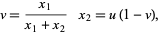
Let

 u=x_1+x_2    x_1=uv

(35)

 v=(x_1)/(x_1+x_2)    x_2=u(1-v),

(36)

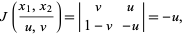
then the Jacobian is

 J((x_1,x_2)/(u,v))=|v u; 1-v -u|=-u,

(37)

so

 g(u,v)dudv=f(x,y)dxdy=f(x,y)ududv.

(38)

g(u,v) = u/(Gamma(alpha_1)Gamma(alpha_2))e^(-u)(uv)^(alpha_1-1)u^(alpha_2-1)(1-v)^(alpha_2-1)

(39)

= 1/(Gamma(alpha_1)Gamma(alpha_2))e^(-u)u^(alpha_1+alpha_2-1)v^(alpha_1-1)(1-v)^(alpha_2-1).

(40)

The sum X_1+X_2 therefore has the distribution

 f(u)=f(x_1+x_2)=int_0^1g(u,v)dv=(e^(-u)u^(alpha_1+alpha_2-1))/(Gamma(alpha_1+alpha_2)),

(41)

which is a gamma distribution, and the ratio X_1/(X_1+X_2) has the distribution

h(v) = h((x_1)/(x_1+x_2))

(42)

= int_0^inftyg(u,v)du

(43)

= (v^(alpha_1-1)(1-v)^(alpha_2-1))/(B(alpha_1,alpha_2)),

(44)

where B is the beta function, which is a beta distribution.

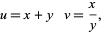
If X and Y are gamma variates with parameters alpha_1 and alpha_2, the X/Y is a variate with a beta prime distribution with parameters alpha_1 and alpha_2. Let

 u=x+y    v=x/y,

(45)

then the Jacobian is

 J((u,v)/(x,y))=|1 1; 1/y -x/(y^2)|=-(x+y)/(y^2)=-((1+v)^2)/u,

(46)

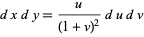
so

 dxdy=u/((1+v)^2)dudv

(47)

g(u,v) = 1/(Gamma(alpha_1)Gamma(alpha_2))e^(-u)((uv)/(1+v))^(alpha_1-1)(u/(1+v))^(alpha_2-1)u/((1+v)^2)

(48)

= 1/(Gamma(alpha_1)Gamma(alpha_2))e^(-u)u^(alpha_1+alpha_2-1)v^(alpha_1-1)(1+v)^(-alpha_1-alpha_2).

(49)

The ratio X/Y therefore has the distribution

 h(v)=int_0^inftyg(u,v)du=(v^(alpha_1-1)(1+v)^(-alpha_1-alpha_2))/(B(alpha_1,alpha_2)),

(50)

which is a beta prime distribution with parameters (alpha_1,alpha_2).

The "standard form" of the gamma distribution is given by letting y=x/theta, so dy=dx/theta and

P(y)dy = (x^(alpha-1)e^(-x/theta))/(Gamma(alpha)theta^alpha)dx

(51)

= ((thetay)^(alpha-1)e^(-y))/(Gamma(alpha)theta^alpha)(thetady)

(52)

= (y^(alpha-1)e^(-y))/(Gamma(alpha))dy,

(53)

so the moments about 0 are

nu_r = 1/(Gamma(alpha))int_0^inftye^(-x)x^(alpha-1+r)dx

(54)

= (Gamma(alpha+r))/(Gamma(alpha))

(55)

= (alpha)_r,

(56)

where (alpha)_r is the Pochhammer symbol. The moments about mu=mu_1 are then

mu_1 = alpha

(57)

mu_2 = alpha

(58)

mu_3 = 2alpha

(59)

mu_4 = 3alpha^2+6alpha.

(60)

The moment-generating function is

 M(t)=1/((1-t)^alpha),

(61)

and the cumulant-generating function is

 K(t)=alphaln(1-t)=alpha(t+1/2t^2+1/3t^3+...),

(62)

so the cumulants are

 kappa_r=alphaGamma(r).

(63)

If X is a normal variate with mean mu and standard deviation sigma, then

 Y=((X-mu)^2)/(2sigma^2)

(64)

is a standard gamma variate with parameter alpha=1/2.


REFERENCES:

Beyer, W. H. CRC Standard Mathematical Tables, 28th ed. Boca Raton, FL: CRC Press, p. 534, 1987.

Jambunathan, M. V. "Some Properties of Beta and Gamma Distributions." Ann. Math. Stat. 25, 401-405, 1954.

Papoulis, A. Probability, Random Variables, and Stochastic Processes, 2nd ed. New York: McGraw-Hill, pp. 103-104, 1984.

اشترك بقناتنا على التلجرام ليصلك كل ما هو جديد